Tutorial
sIArena is a Python project that provides a simple and easy-to-use interface to test path finding algorithms. It is able to generate pseudo-random maps called Terrain to simulate a 2D environment.
A Terrain is a 2D grid of cells formed by an integer matrix, a point of origin and a point of destination. Each cell of the matrix represents the height of that cell, what it is used to calculate the cost of moving from one cell to another. A Path is a list of Coordinates that represents a path from the origin to the destination of a specific terrain. These path could be measured to determine the total cost of moving from the origin to the destination. As lower the cost, better the path.
This project implements the environment required to test different path finding algorithms and compare their performance in path cost and time. It provides generation tools to create pseudo-random terrains, visualization tools to display terrains and paths in a graphical interface, and measure tools to measure algorithm performance.
Installation
sIArena is a Python project, check the following section to install the project and its dependencies.
The advised way to install sIArena is using a Python Jupyter Notebook in Google Colab, or using a package manager like pip or Anaconda in a local environment.
Generate a terrain
In order create a path finding algorithm, first we need to create a terrain to test it. The library provides a set of tools to generate pseudo-random terrains.
The following snippet generates the terrain displayed below.
from sIArena.terrain.Terrain import Coordinate, Terrain, Path
from sIArena.terrain.generator.PerlinGenerator import PerlinGenerator

terrain = PerlinGenerator().generate_random_terrain(
    n=25,
    m=25,
    min_height=0,
    max_height=100,
    min_step=25,
    abruptness=0.1,
    seed=60,
    origin=None,
    destination=None)

# To print the terrain in ascii format
print(terrain)
We can see printed the terrain matrix.
The origin cell is represented by a +, and the destination cell by a x.
Plot the terrain
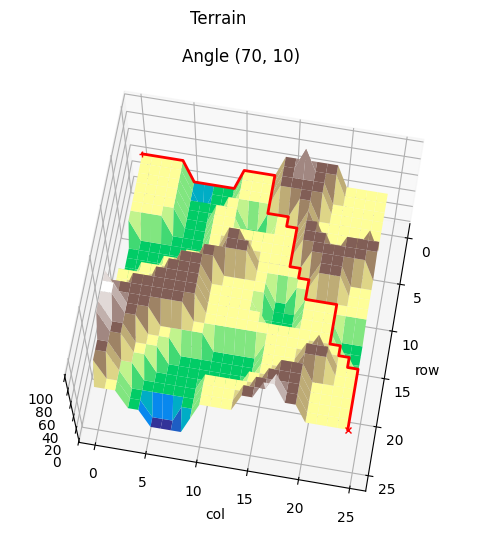
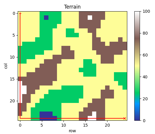
The terrains could be graphically displayed using the plotting tools. These tools allow to display the terrain as a height map in 2D or 3D.
The following snippet plots the terrain generated in the previous section:
from sIArena.terrain.plot.plot_2D import plot_terrain_2D
from sIArena.terrain.plot.plot_3D import plot_terrain_3D

plot_terrain_2D(terrain)
plot_terrain_3D(terrain, angles=[(80, 10), (30, 190), (30, 10)])


Path finding algorithm
The main goal of the library is to allow to create and test different path finding algorithms. These algorithms are expected to find the lowest cost possible path from the origin to the destination of a terrain. To generate such kind of algorithms, just create a function which only parameter is a terrain, and that returns a path.
A path is a list of sequently Coordinates from the origin to the destination of a specific terrain. In order for a path to be valid, each coordinate must be adjacent to the next one, this means, to be at a distance of 1 in the x or y axis, but not in both at the same time.
The following snippet shows different methods from terrain that could be useful to build the path finding algorithm:
# Get the terrain size
n, m = terrain.size()

# Get origin and destination coordinates
origin = terrain.origin
destination = terrain.destination

# Check the possible neighbors of the origin (thus, the possible next step of the path)
neigs = terrain.get_neighbors(origin)

# Check the cost from the origin to each neighbor
costs = [terrain.get_cost(origin, neig) for neig in neigs]
In order for a path to be complete, the first coordinate must be the origin and the last one the destination. The following snippet shows different a path finding algorithm that goes down to the end of the map, and then right. Be aware that not all the terrains start and end in the corners, but their origin and destination may vary.
from sIArena.terrain.Terrain import Coordinate, Terrain, Path

def find_path(terrain: Terrain) -> Path:

    # Create a path that starts in origin
    path = [origin]

    # Go to the buttom of the map (assuming destination is in [N-1,M-1])
    for i in range(n-1):
        path.append((path[-1][0] + 1, path[-1][1]))

    # Go to the right of the map (assuming destination is in [N-1,M-1])
    for i in range(m-1):
        path.append((path[-1][0], path[-1][1] + 1))

    # Return the path
    return path
And in the following some methods to check the path and its cost:
# Get the path solution
path = find_path(terrain)

# Check if a path is complete (it must be with our implementation)
is_complete = terrain.is_complete_path(path)

# Calculate the cost of a path
cost = terrain.get_path_cost(path)

print(f"The path {path} with cost {cost} {'is' if is_complete else 'is not'} complete.")
Plot the path
The library also support to show a path in the terrain, as shown in the following snippet:
from sIArena.terrain.plot.plot_2D import plot_terrain_2D
from sIArena.terrain.plot.plot_3D import plot_terrain_3D

plot_terrain_2D(terrain, paths=[path])
plot_terrain_3D(terrain, paths=[path], angles=[(80, 10), (30, 190), (30, 10)])

Measurement
The library also provides a way to measure the performance of the path finding algorithms. This is done by measuring the mean time and the minimum cost of the path found by the algorithm over a terrain.
The following snippet shows how to measure the performance of the algorithm implemented before:
from sIArena.measurements.measurements import measure_function

min_cost, second, min_path = measure_function(
    find_path,
    terrain,
    iterations=5,
    debug=True)

print(f"Minimum cost: {min_cost} found in {second} seconds:\n{path}")
The previous algorithm finds in fractions of milliseconds a path with cost 559.
Conclusion
Creating a terrain, and the testing a path finding algorithm is a simple and easy task using sIArena. Knowing the time needed to find a path, and the cost of it, different algorithms could be compared to determine which one is the best for a specific terrain.
For instance, in the map generated before,
the lowest cost path should look like the following, with cost 121: